
Author: Loren Oki, UC Davis Department of Plant Sciences
A Step by step guide with example problems to determine how long to run your irrigation system.
Measuring Distribution Uniformity and Calculating Run Time
Steps to determining distribution uniformity
A. Collect measurements
- Make a map of the irrigated are and the drip system.
- Set up containers under emitters to collect water. It doesn’t matter what kind of container you use for a drip system. (This is not true if you are measuring microsprays!)
- Note their locations on the map.
- Use a quantity of containers that is evenly divisible by 4. That is 24, 36, or 40, for examples. Use at least 24 containers. More is better, but you shouldn’t need more than 40.
- Place the containers evenly along and across the drip system. Include containers close to and far from the valve. Note where the containers are on your map.
- Collect water in the containers. Be careful to not overtop the containers!
- Make sure you record the run time.
- Measure the water volumes in milliliters (mL). Ounces (oz.) will work, but there is more accuracy with mL. If you use one of my spreadsheets, you must use mL.
- Record the measurements. The map may be helpful to be able to trace the volume back to the location of the container if problems appear.
B. Calculate Distribution Uniformity (DU)
- Sort the list of volumes from largest to smallest.
- Calculate the average of the lowest quartile (AvgLQ). If you have 36 volumes, that would be the average of the lowest 9 measurements.
- Calculate the average of all of the measurements (total average or AvgT).
- Divide the average of the lowest quartile (AvgLQ) by the total average (AvgT) to get distribution uniformity (DU).
Calculation #1:

C. You can also use a spreadsheet to calculate DU.
The DU value tells us how evenly the water is being applied to the irrigated area. A DU of 1.0, which is impossible to get, would mean that every emitter is delivering the same amount of water during an irrigation. Drip systems can deliver water with very high DU, in the 0.8s and 0.9s. When a system has a DU of 0.7 or less, maintenance is necessary.
Calculating Run Time
The information that you need to calculate run time for a drip irrigation system is:
- The “precipitation rate” of the system
- The soil type
- The depth that you want to wet the soil
- The scheduling multiplier
Precipitation (Application) Rate
Water application rates for irrigation systems are typically given in inches per hour (in/hr) , but drip system application rates are in gallons per hour (gph). So, we’ll have to convert the drip rate to inches per hour.
Method 1
We need to know:
- Area irrigated (sq ft)
- Total number of emitters in the irrigated landscape area
- Emitter flow rate (gph). This is the flow rate for each emitter
Calculation #2:

There are two places where we can get the flow per emitter number. The flow rate specified on the product is easy to get and is usually molded into the emitters. For accuracy, we can also use the information from the DU assessment we conducted earlier. But it means more math:
Calculation #3:

Method 2 for inline drip tube
We need to know:
- Emitter flow rate (gph) (This can found printed on the tube, obtained from the manufacturer, or from a calculation using the DU values and the formula above)
- Emitter spacing on tube (usually 12” or 18”)
- Lateral spacing (space between tubes) in landscape (usually 12”, 14” or 16”)
Calculation #4:

Soil Water Holding Capacity
We need to know how much water the soil can hold before we can determine how long to run the irrigation. To do this, we need to know the texture of the soil. The “easiest” way to get this information is to use a smartphone and an app called: “SoilWeb” that is available from UC Davis at: http://casoilresource.lawr.ucdavis.edu/soilweb-apps/
The information we need is in the section “Available Water Storage (0-100cm)” and is usually in cm. Divide the value listed by the depth provided (in this case “100”) to give us the Plant Available Water (PAW) that we’ll use in the runtime calculation.
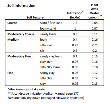
Another way to estimate this number is to identify the soil type and use the Soil Information table. Find the soil type of the site and use the corresponding value in the “Plant Avail Water (cm/cm)” column.
Depth to Wet
Another number needed is the depth the water needs to be wetted. Soil under turf should be wetted to 12” and this would also include flower beds and most groundcover. Larger shrubs should be wetted down to 18”. Trees tend to be planted among turf, ground cover, and shrubs and receive the irrigation given to the smaller plants. However, if the irrigation to the smaller plants is reduced or turned off, be sure to provide irrigation to the trees down to 24” or deeper occasionally.
Another Calculation first...
We need to account for the uniformity of the irrigation system in the run time calculation and we’ll use the Distribution Uniformity (DU) determind earlier to calculate the Scheduling Multiplier (SM).
Calculation #5:

Calculating Run Time
To calculate the run time (hours) we need to know:
- Depth to wet the soil (inches)
- Plant available water in the soil
- Application rate of the irrigation system that was calculated in a previous step
Calculation #6:
![]()
This will give us the number of hours to run the irrigation to wet the soil down to the desired depth. This value can be programmed into an irrigation controller.
Example Calculations
In this example, the area is a 400 square foot bed of low ground cover and small herbaceous perennials irrigated by the drip system. There are 415 point source emitters with a flow of 0.6 gph. The soil is a Yolo silty clay loam and Soil Web indicates the Available Water Storage in 100 cm of soil is 18.7 cm.
DU container volumes collected: 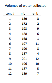
- (You should use at least 24 containers. I’m using only 12 in this example).
- Run time = 5 minutes
The container volumes collected are in the table to the right. The “rank” column indicates the order of volumes from smallest to largest.
Distribution Uniformity
- Calculate the overall average (AvgT). Add all of the values and divide by the number of values. The total of the mL column is 2248 and dividing that by the number of measurements gives: 2248/12=187.3= AvgT. (Calculation #1)
- Rank the values in order and calculate the average of the lowest quartile (AvgLQ). The lowest 3 numbers (in bold) add up to 520 and when divided by 3 gives: 520/3=173.3= AvgLQ.
- DU is determined by dividing AvgLQ by AvgT and results in: 173.3/187.3= 0.93= DU.
Precipitation (Application) Rate
4. The precipitation rate is determined using Calculation #2 and:
a. Area irrigated is 400 sq ft.
b. The number of emitters is 415
c. The flow rate is 0.6 gph
5. So, the formula is: Application Rate = 415 × 0.6 × 1.604 / 400 = 1.0 inches per hour
6. If we wanted to calculate the flow per emitter based on the volumes collected in the DU assessment, this would be done using Calculation #3:
a. AvgT is 187.3
b. Run time is 5 minutes
7. So, this calculation is: Flow per emitter = 187.3 / 5 / 63.08 = 0.59 gph
8. If we were using inline drip tube, we could calculate the application rate a different way. The tubing in this example has 0.6 gph emitters spaced 12 inches on the tube and the tube was installed with 12 inches between the tubes, using calculation #4 would use be: Application Rate = 0.6 × 231.1 / 12 / 12 = 0.96 inches per hour which is really close to (and essentially the same as) the value calculated in line #5 above.
9. Now we need to determine the scheduling multiplier using calculation #5:
a. Our DU is 0.93 so the calculation is: Scheduling multiplier = 1/ (0.4 + (0.6 × 0.93)). This one is a little trick and you need to do the separate operations in a specific order:
i. 0.6 × 0.93 = 0.558
ii. 0.4 + 0.558 = 0.958
iii. 1 / 0.958 = 1.04 = Scheduling Multiplier
Run Time
10. First we need to know the depth to wet and how much water the soil holds. Since this is a bed of low ground cover and small herbaceous perennials, the desired wetting depth is 12 inches. SoilWeb showed us that the Available Water Storage in 100 cm of soil is 18.7 cm. We need to divide the 18.7 cm by 100 cm and that gives us 0.187 which we can round to 0.19. Now we have what we need to calculate the run time for the valve:
Using Calculation #6: Runtime = 12 × 0.19 / 1.0 / 1.04 / 2 = 1.096 or 1.1 hours
11. Irrigation controllers accept run times differently and probably don’t accept the decimal hours: we can’t enter 1.1 hours as a run time. So we need to convert this to hours and minutes or minutes. Hours and minutes: is 1 hour and 0.1 × 60 = 6 minutes. Now you can enter 1:06 if your clock accepts hours:minutes.
For minutes only, 1.1 hours = 1.1 × 60 = 66 minutes
12. DONE!
13. Something to note: See that we calculated the application rate as 1.0 inches per hour? Now look at the chart of soil information for the silty clay loam soil for our example and look what the infiltration rate is (0.05 in/hr). This is the rate that the soil will absorb the water and it is much lower than the rate the water is being applied. So we need to watch for runoff. If runoff appears during irrigation, then the application will need to be divided into several shorter “pulses”. To determine how long the pulse should be, wait until an irrigation is needed and then turn on the valve. Wait until runoff starts and then turn off the water, noting how long that took. If runoff appeared after 11 minutes, then you’ll have to apply 6 pulses of 11 minutes each for a total of 66 minutes to apply the proper amount of water and avoid producing runoff!
Literature and other information sources used
Costello, L.R. and K.S. Jones. 2014. Water Use Classifications of Landscape Species. WUCOLS IV. California Department of Water Resources, the University of California, and the California Center for Urban Horticulture (UC Davis). https://ccuh.ucdavis.edu/wucols.
Landscape Irrigation Auditor Second Edition. 2011. Irrigation Association. Falls Church, VA
McCabe, J. (ed). 2010. Turf and landscape irrigation best management practices. Irrigation Association Water Management Committee. http://www.irrigation.org/uploadedFiles/Resources/BMP_Revised_12- 2010.pdf.
Schwankl, L., F. Lamm, and D. Porter. Maintenance of microirrigation systems. Division of Agricultural and Natural Resources University of California. http://micromaintain.ucanr.edu/. Accessed 2016Sep30.
Shaw, D.A. and D.R. Pittenger. 2009. Landscape irrigation system evaluation and management. University of California, Cooperative Extension. http://ucanr.org/sites/urbanhort/files/80223.pdf.
By Loren Oki 2016Sep30